The KinExA platform can be used to determine unknown sample concentrations with a high level of sensitivity and accuracy. Relatively large molecules can often be directly measured using a “Sandwich” assay. In cases where a sandwich assay is not feasible, e.g. small molecules, an inhibition assay can be performed. This document provides an overview of how to set up and evaluate both assay formats using KinExA technology.

For either method, a standard curve is defined using known sample concentrations. The unknowns are measured under the same conditions, and signals from the unknowns are converted to concentration using the standard curve (Figure 1).

Any standard curve will have a useful measurement range (the “dynamic range”) in the middle of the curve, and unknowns above or below this range will not be accurately quantified.

The basic concept of the dynamic range can be easily understood by considering the effect of measurement reproducibility or noise. Figure 2 shows a standard curve and 3 measured signals with error bars indicating the uncertainty in signal. For the point in the middle of the curve, the uncertainty transforms into a relatively narrow range of concentrations indicated by the width of the vertical shading on the concentration axis. Notice that the steeper the slope of the response curve the narrower the range of concentrations. On the other hand, as we near either plateau of the standard curve the same degree of measurement noise (the same exact size of error bar) leads to concentration ranges that are much wider. If you imagine sliding one of the error bars along the standard curve you can envision the concentration range changing from infinitely wide to narrow and then back again.

As an analyst it is important to understand the influence your assay’s reproducibility has on the precision of your concentration estimate. In many cases a general understanding as described here may be enough. If it is desirable to quantify the dynamic range, a good reference is Hayashi¹ in which the calculation of the dynamic range and least detectable concentration is formalized in a way that allows comparisons between different assay formats and platforms².

IMPORTANT NOTE: The KinExA Pro software will report values for unknowns that are outside the dynamic range of the assay. If the percent free value reported for an unknown is greater than 90% or less than 10% it is important to consider your system noise before accepting the result.

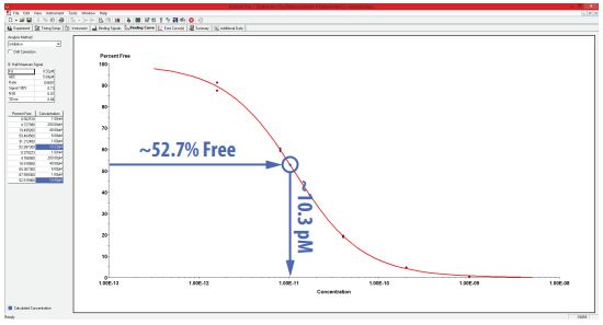
Figure 1. Standard curve to calculate concentration from measured signal.

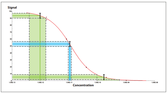
Figure 2. Measurement noise (vertical error bars) leads to very different concentration uncertainty depending on the slope of the standard curve at the measured concentration.

Inhibition Immunoassay

For this assay format the analyte (or a cross reacting analog of it) is immobilized on the solid phase. The detection antibody is mixed with the sample, allowed to equilibrate, and flowed through the solid phase. Presence of the analyte inhibits binding of the detection antibody to the solid phase. The analyte concentration is determined by comparison to a standard curve constructed using known concentrations of analyte and detection antibody. The KinExA Pro Inhibition analysis method uses an exact solution of the bimolecular binding equation to fit the standard curve. The unknowns are then interpolated.

Optimum sensitivity and dynamic range for this assay format is achieved by using a K_d controlled standard curve³. Acquiring accurate measurements also depends on knowing the active concentrations of the binding partners. Once the K_d and activity are known the theory curve can be used to find a concentration of antibody that gives a satisfactory range and sensitivity.

Figure 3 shows 3 calibration curves, each with a different antibody concentration. The K_d of the antibody is 5 pM so a 1 nM antibody concentration gives a concentration controlled curve with a narrow range of measurable concentrations (because of the steep slope) and a relatively insensitive least detectable concentration (because of the curve’s placement). The advantage of this curve is that it comes to equilibrium quickly and the high antibody concentration means fast easy measurements. On the other hand, a 1 pM antibody concentration gives a K_d controlled curve and its characteristic shallow slope results in a larger dynamic range while its position on the analyte axis (50% inhibition ≈ K_d) gives the lowest analyte detection limit. The disadvantage here is the samples will take longer to equilibrate, the low antibody concentration will require larger volumes of sample, and the measurement time will increase. The choice of which curve to use will usually be governed by the sensitivity required. Curves between the extremes offer a compromise in terms of time, sample volume, and sensitivity.

It should also be mentioned that if the least detectable concentration requirement is less than the K_d divided by 10 then detection will be difficult. Whenever possible an antibody with a K_d near or below the assay’s target sensitivity should be chosen.

To maximize accuracy it is important to make up and run the unknown samples at the same time as the standard curve. This reduces the error that can be caused from different experimental conditions.

Figure 3. The theoretical binding curve showing binding curves for various CBP concentrations for the same K_d value.

Inhibition Analysis

Once the experiment is complete the concentrations can be calculated using the Inhibition analysis method under the Binding Curve tab. Using the signals generated the percent free CBP is calculated and then plotted against known analyte concentrations, generating a standard curve. The unknown samples will be placed on the standard curve depending on the calculated percent free CBP for each unknown. The analyte concentrations can then be determined depending on where the unknown falls on the curve (Figure 4).

Figure 4. Inhibition method of finding an unknown analyte concentration using the percent free constant binding partner and a standard curve.

“Sandwich” Immunoassay

A sandwich assay requires the analyte to have two distinct binding epitopes that can be simultaneously bound by two antibodies. The KinExA solid phase is coated with the first antibody which captures the analyte by binding to one of the epitopes. Detection of the captured analyte is accomplished by binding a fluorescently labeled antibody to the second epitope. Unknown concentrations are determined from a standard curve. It is recommended that the range of standards used encompass the unknowns, that is, that the unknowns be interpolated rather than extrapolated.

Creating an Optimal Standard Curve

Optimization should include generating signals using standards spanning the desired working range of the assay. Factors to consider in the optimization include primary vs secondary labeling, choice of which antibody to immobilize, choice of solid phase for immobilization, cost of reagents, and the time required to run the assay. Other considerations include the volume and flow rate for the sample, detection antibody, and secondary labeling antibody, if used. Once a promising set of factors are identified, running two to four points in the desired range will be adequate to determine the unknown sample’s concentration.

Sandwich Analysis

Once the experiment is run, the concentrations can then be calculated using the Sandwich analysis method under the Binding Curve tab.

The data is fit using the following hyperbolic equation:

In this equation A is equal to the maximum saturation signal and B is the concentration that gives half the maximum signal. Figure 5 is an example of a Sandwich analysis where A equals 21.13 and B equals 2.30 nM. The unknown concentration is shown in blue.

Figure 5. Example of a Sandwich analysis in the KinExA Pro software.

Software Setup

Open a new KinExA equilibrium experiment from the templates. On the Experiment page, select Concentration Measurement under the Experiment Type drop down. When entering concentrations on the Timing Setup page enter the standard and unknown samples in the Titrant Concentration column under Sample Timing. For the unknown samples, place a question mark in the column so that the KinExA Pro software knows which sample concentrations to calculate. Once the experiment is complete choose the appropriate analysis method, inhibition or sandwich, and analyze the results.

Conclusion

In immunoassay, the dynamic range and least detectable concentration are ultimately limited by the properties of the antibodies used. However, not all immunoassay measurement technology is able to achieve the full potential of the antibody. By avoiding competition and providing excellent fluorescent sensitivity (low to sub pM) the KinExA system has been shown to routinely take full advantage of even extremely tight binding antibodies³. This makes the KinExA an ideal tool for measuring unknown samples.

References

1. Hayashi, Y., et al. 2004. Precision, limit of detection and range of quantitation in competitive ELISA. Anal Chem 76:1295-1301. http://www.ncbi.nlm.nih.gov/pubmed/14987084
2. Glass T.R., Ohmura N., Saiki H. 2007. Least detectable concentration and dynamic range of three immunoassay systems using the same antibody. Anal Chem 79: 1954-1960.
3. Ohmura N., Lackie S., Saiki H. 2001. An immunoassay for small analytes with theoretical detection limits. Anal Chem 73: 3392-3399. http://www.ncbi.nlm.nih.gov/pubmed/11476240