Newsletter #2

Whole Cells
The flexibility of the KinExA® instrument allows the measurement of both soluble and membrane-bound molecules. When performing a whole cell experiment, the whole cells take the place of the titrant in the standard KinExA assay.
Cells are titrated in a background of the constant binding partner. When titrating the cells, the highest concentration should be approximately 2 orders of magnitude greater than the Kd so the bottom of the curve is fully saturated. Typically, the Kd is unknown so starting at the maximum practical concentration of cells, and including a large number of dilutions of the cells, will increase the chance of success. If you have an idea of the expression level, the dilution series should go down to an effective concentration of about 1 to 10% of the constant binding partner concentration (see Table 1).
Table 1. Serial Dilutions for 10 Million Cells at Differing Cellular Expression Levels
| Max Cells/mL | Binding Sites/Cell | Molar Equivalent of Cells | Maximum Kd Value | Number of 2-Fold Serial Dilutions | Number of 3-Fold Serial Dilutions |
|---|---|---|---|---|---|
| 1.00E+07 | 10,000 | 1.66E-10 | 1.66E-12 | 11 | 7 |
| 1.00E+07 | 100,000 | 1.66E-09 | 1.66E-11 | 14 | 9 |
| 1.00E+07 | 1.00E+06 | 1.66E-08 | 1.66E-10 | 17 | 11 |
| 1.00E+07 | 1.00E+07 | 1.66E-07 | 1.66E-09 | 20 | 13 |
Table 1. Number of 2-fold and 3-fold serial dilutions suggested for 10 million cells at differing cellular expression levels.
When the cell titration series reaches equilibrium, the solutions are centrifuged. The supernatants are then removed and conserved. The supernatants contain only the free constant binding partner, thus allowing the use of either a soluble whole cell receptor/titrant or an anti-species antibody as the capture reagent (Figure 1). The cell-free solutions are run through the KinExA instrument and the expression level is calculated.
Whole cell analysis is a variant of unknown titrant analysis, therefore two curves are needed to resolve the Kd and the expression level. Usually completing one curve at a higher and one at a lower constant binding partner concentration and then using the n-curve analysis will accomplish this. Since the cell expression level can drift, it is important that both curves be run using the same batch of cells at the same time. For more information on completing a whole cell experiment please refer to Technical Note TN211 (Whole Cell Assay).
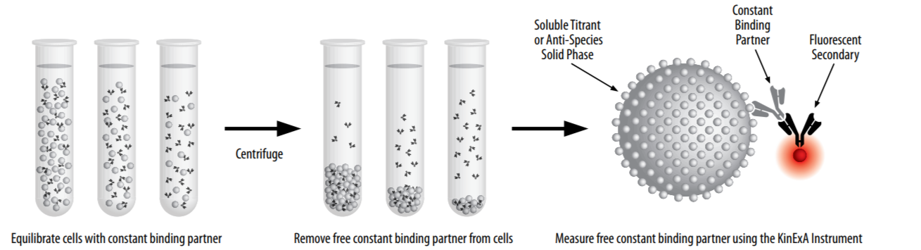
Figure 1. Illustration of whole cell setup.
How Low Can We Go?
 A new Microtiter Plate Sample Rack (Part #: 414106) has been developed as an accessory to the Autosampler. This rack supports the use of 96 sample microtiter plates and the custom 48 Sample Microcentrifuge Racks (Part #: 21148 from Syringa Lab Supplies). With the ability to use small volume microtiter plates and sample tubes, we wanted to know the minimum sample volume for experiments, and the minimum dead volume required.
Minimum Sample Volume
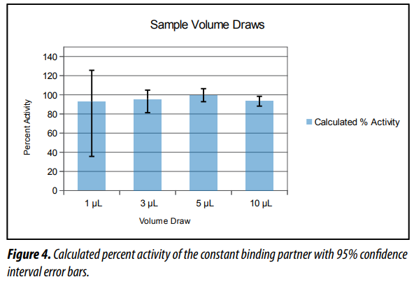
First, we determined the minimum sample volume for experiments. Four separate experiments were set up using 1 μL, 3 μL, 5 μL, or 10 μL sample draws. The “concentration controlled” curves generated were suitable for measuring the Active Binding Site Concentration (ABC). The activity for the constant binding partner was calculated by dividing the measured ABC by the nominal binding site concentration. Figure 4 shows the calculated percent activity for each experiment.
Although 1 μL can be used successfully, slightly larger (3 or 5 μL) sample volumes should be used to decrease the error, which will give greater confidence to the measurement.
Minimum Dead Volume
The minimum dead volume required was determined by using small volume tubes (Part #: 22015 from Syringa Lab Supplies) covered with a sealing film (Part #: 20030 from Syringa Lab Supplies) in a 48 sample micro-centrifuge rack. These tubes are specially made to closely fit the diameter of the sipper tube, allowing immersion of the tip inlet in a minimum volume of liquid. Experiments were set up for 5 μL sample draws in duplicate, with additional “dead” volumes of 8 μL, 10 μL, or 13 μL.
Bubbles were introduced during the second run for the 8 μL dead volume test which resulted in the large 95% confidence interval (Figure 5). Based on these results, 10 μL of dead volume is sufficient for the amount of time it took to run this experiment (~5 hours). If possible, slightly more dead volume is suggested to avoid the effects of evaporation.
For more information about this, refer to Tech Note TN206 (Minimum Sample Volume).

Spotlight: Siliconized Flow Cells
Running sticky systems through the KinExA instrument can result in unwanted adsorption to the flow cell. This is most commonly seen as baseline creep and/or titrant related non-specific binding (TR NSB). In an effort to reduce these effects, Sapidyne Instruments has developed the Siliconized Flow Cell (Part #: 392150). The siliconized flow cell is coated with a layer of octadecyltrialkosilane on the glass to reduce surface adsorption.
Baseline Creep is caused by one or more reagents binding to the sides of a non-siliconized flow cell. With each additional run, reagents continue to build up and the baseline signal increases.
TR NSB is caused when high titrant concentrations exhibit a positive slope on the binding curve where normally the slope should be nearing zero.
In either case, using a siliconized flow cell can reduce these effects and narrow the confidence intervals. These flow cells are an excellent option for systems where baseline creep or TR NSB have become a problem. See Tech Note TN210 (Titrant Related NSB) and Tech Note TN216 (Baseline Creep) for more information.
Ask the Inventor
Question
What do the KinExA error graphs show and how should they be used?
Answer
The KinExA error graphs show a plot of the residual error when the selected binding theory is fit to the measured data for a series of fixed Kd values (Kd error graph) or fixed ABC values (ABC error graph). The graphs provide a useful visual indication of whether your experiment succeeded in resolving the Kd and ABC values.
Explanation
When you click “analyze” the KinExA Pro software finds values for the Kd, ABC, Sig100, and NSB that give a minimum RMS (square Root of the Mean Square) error between the theory and the measured data. The error is computed as the difference between the measured data at a given concentration and the theoretical value at the same concentration. Following standard practice, the errors are squared, then averaged, and the square root is taken. After the Kd, ABC, Sig100, and NSB are optimized, meaning the RMS error is minimized, the error still remaining is called the residual error.
The “Binding Curve” tab in the KinExA Pro software reports the optimum Kd, ABC, Sig100, and NSB values along with the residual error labeled “%Error”. While the “Binding Curve” tab gives the optimum Kd (for example) the “Error Curves” tab answers the question “what other Kd’s fit nearly as well?”
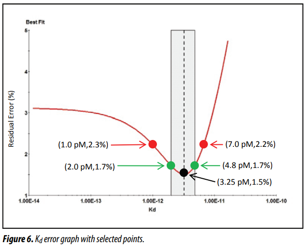
The Kd error graph is constructed by fixing the Kd at a series of values on both sides of the optimum then finding the residual error after optimizing the values of the ABC, Sig100, and NSB, without varying the Kd. The optimum Kd and the residual %Error reported on the “Binding Curve” tab correspond to the coordinates of the minimum value on the error graph. What we hope is that the error graph has a sharp well defined minima, with the residual error increasing rapidly as the Kd moves away from the optimum value.
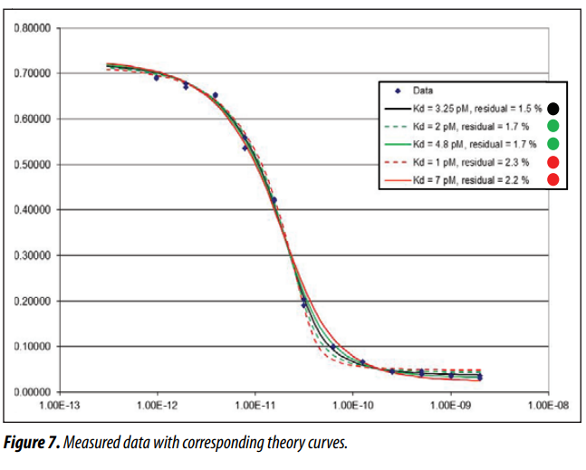
Figure 6 shows a Kd error graph annotated with coordinates of 5 selected points. The 95% confidence interval (CI) is shown by the shaded region and extends from 2 pM to 4.8 pM. Figure 7 shows the measured data, along with the best fit of the theory, corresponding to the 5 selected points in Figure 6.
The black line in Figure 7 is the best fit of the theory to the data and the optimum Kd value found in the fitting is 3.25 pM. The green dashed line shows the best fit found with the Kd fixed at 2.0 pM and the green solid line shows the theory fit with the Kd fixed at 4.8 pM. Both green lines are still a good fit to the data, consistent with the idea the true Kd could be anywhere in this range. The fit at 1 pM and 7 pM are noticeably worse and lay outside the 95% CI.
The width of the confidence interval is computed by finding the corresponding Kd values that increase the residual error to the cutoff level. The cutoff level for a 95% confidence interval was determined from a large number of Monte Carlo simulations which are described in more detail in Tech Note TN207 (KinExA Error Curves and the 95% Confidence Interval).
Hints & Tricks
Lamp Alignment and the EPM
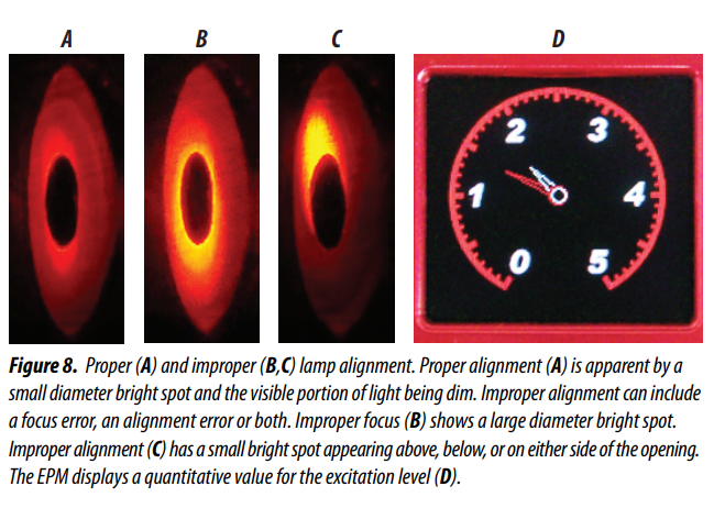
The lamp in your KinExA instrument provides the excitation for the fluorescent label your system uses to provide a signal. Proper alignment of the lamp maximizes excitation, giving optimum signal. Customer feedback has led us to develop a new tool, the Excitation Power Monitor (EPM), to assist in this procedure.
There are now two ways to align the lamp. See How to Guide HG204 (Lamp Replacement and Alignment) for instructions. Both methods use the same procedure for adjusting the lamp, however, the way in which you determine best placement is different:
- Subjectively, using the lamp alignment window. This is the original method where you look at a pinhole and attempt to focus and align the lamp against it. People have found this method difficult and confusing. This can be a source of trouble as it is possible for a user to improperly align the lamp, yet have no way of knowing anything is wrong (Figure 8A–C).
- Empirically, using the new Excitation Power Monitor. The EPM measures excitation levels directly at the flow cell, allowing users to quickly adjust the lamp to maximum signal with confidence (Figure 8D).
The EPM was developed to help KinExA users correctly align the lamp to achieve optimal signal. It eliminates ambiguity and uncertainty in KinExA lamp alignment. This new system gives scientists a quantitative value for the brightness of the light at the flow cell, while making lamp adjustment a snap!
EPM Advantages
- Quickly and easily maximize signal levels
- Quantitative measurement of actual excitation power at the flow cell
- Bright, colorful display shows both current and peak readings at a glance
Features
- Simple user-interface
- Small, light-weight, hand-held design
- Powered through the lamp connection; no batteries to replace
- Comes with a custom padded storage case
Store Your Results
- Saves excitation values across multiple instruments and lamp changes
- Built in memory can permanently store hundreds of readings
- Track excitation power over the lamp’s life