
Newsletter #3

Theory Curve
The Theoretical Binding Curve Demonstration Tool “Theory Curve” is a KinExA Pro application designed and maintained by Sapidyne Instruments Inc. The Theory Curve is based on the reversible binding equation (eq. 1) describing the binding between two molecules in solution.
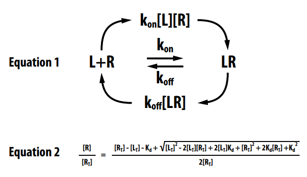
Interacting with this tool helps develop an understanding of bimolecular interactions that are not readily apparent from the bimolecular binding equation or its solution (eq. 2). The Theory Curve can be used when modeling solutions where one of the binding partners has a fixed concentration (Constant Binding Partner or CBP) and the other binding partner’s concentration is varied (Titrant). When opening the application you will see a graph displaying the percentage of CBP that is free at equilibrium (Y axis) as a function of the total titrant concentration (X axis). This graph is interactive so you can change the conditions by sliding a control, and seeing the effect it has on the graph.
Three interactive binding curves are available: Equilibrium, Kinetics Pre-Equilibrium, and Kinetics Time Course.
Equilibrium
Equilibrium models reversible binding at equilibrium. Once equilibrium is achieved the percentage of CBP that is free will remain the same for a given titrant concentration. The percentage is determined by the Kd and the concentrations of the two molecules. Particular experimental conditions will display more sensitivity to either the Kd or the concentration of CBP. Low ratio curves (CBP/Kd < 2) are affinity driven and will be sensitive to the Kd while high ratio curves (>20) are driven by stoichiometry and are more sensitive to the CBP concentration.
Kinetics Pre-Equilibrium
Kinetics Pre-Equilibrium models a full binding curve at a single time point. The dashed line is the equilibrium binding curve. The time slider can be used to vary the time point to see the effect it has on the binding curve.
Kinetics Time Course
Kinetics Time Course models the approach to equilibrium for a reversible binding system. While the Y-axis still displays the percent free CBP, the X-axis now displays time. The dashed line shows where the system will be at equilibrium. The interactive sliders can be used to help understand how the time to equilibrium is affected by concentration or kinetic constants.
Utilizing these tools in planning experiments can save both time and materials. Many also find the simulator useful in understanding and teaching binding theory. For a complete guided tour on how to operate and understand the Theory Curve, please see Tech Note 220 Theory Curve (TN220).
Autosampler Manual Kinetics Direct
Some systems reach equilibrium too quickly to be measured using the Kinetics Direct experiment. Without an Autosampler, the only option is to use the Kinetics Injection experiment. The Injection experiment, however, uses more material and is not as simple. When an Autosampler is available, an Autosampler Manual Kinetics Direct experiment can be used, retaining the advantages of the Kinetics Direct.
One limitation of the Kinetics Direct is that it requires bead handling and time for charging sample lines prior to flowing the first sample. The first point therefore takes 400 to 500 seconds and each subsequent point must wait an entire run (usually 600 to 800 additional seconds) before being sampled.
When using the Autosampler, the sample line does not need to be charged and the bead handling can be done prior to mixing the sample. This allows the first sample to be run within a few seconds after sample mixing. Furthermore, by mixing each sample individually the successive data points can be much closer together filling in gaps that would otherwise exist in a Kinetics Direct curve.
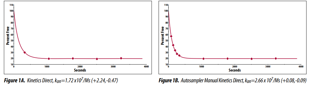
Figure 1A shows an example of a Kinetics Direct experiment that reached equilibrium quickly and did not clearly define the upper part of the curve (kon = 1.72 × 10⁷/Ms, +2.24, −0.47). Figure 1B shows the same system utilizing the Autosampler Manual Kinetics Direct time points. The additional points narrow the confidence interval significantly giving more confidence to the data (kon = 2.66 × 10⁷/Ms, +0.08, −0.09).
For more information on how to perform this experiment, refer to How to Guide 244 Autosampler Manual Kinetics Direct (HG244).
Hints & Tricks
Capture Percentage and Experiments
The KinExA Pro software uses a 1:1 binding model in which the signal is proportional to the free binding sites. However, the most common measurements with kinetic exclusion assays are bivalent IgGs. When a bivalent molecule is detected it gives the same signal whether it had one or two sites free in solution. Therefore, the signals generated directly reflect the number of captured free antibody molecules rather than captured free binding sites.
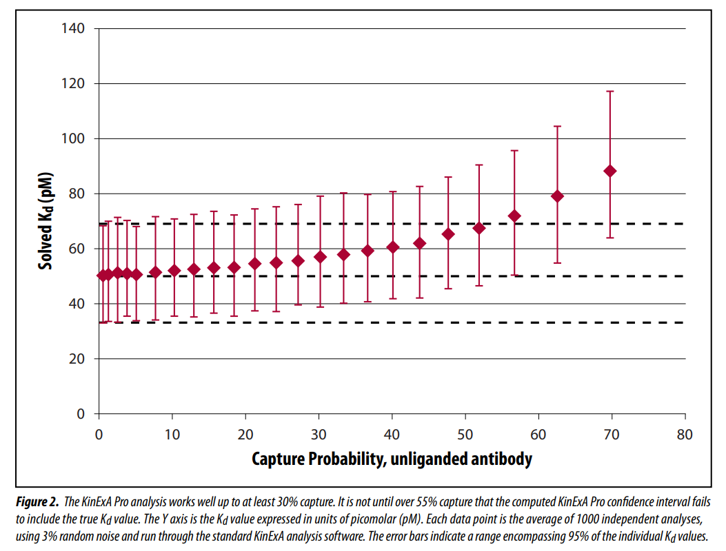
Although the signal from the captured antibody is independent of the number of free binding sites, the probability of an antibody being captured is affected by the number of free binding sites. If the capture probability is low then the signal becomes proportional to the free antibody binding sites in the sample1. Simulations show that high capture may lead to a bias in the Kd measured for multivalent receptors (Figure 2).
Capture probability can easily be measured. The procedure consists of conducting two signal tests using the same beads, flow rate, samples and label while varying bead column heights. The first signal test is run using a standard bead column height while the second signal test uses double the standard bead height.

At the standard KinExA flow rate of 0.25 mL/min the capture percentage is typically low1–3. The capture probability is a function of flow rate: higher flow rates reduce the capture probability and lower flow rates increase it. Users are advised to exercise caution and check the capture in questionable cases such as when unexpectedly large binding signals occur or when using low flow rates.
For a more in-depth and detailed explanation of capture percentage and how it impacts experiments, refer to Tech Note 200 Receptor Valency (TN200).
References
- Glass, T.R., Winzor, D.J. 2014. Confirmation of the validity of the current characterization of immunochemical reactions by kinetic exclusion assay. Anal Biochem 456:38–42
- Blake, R.C., Pavlov, A.R., and Blake, D.A. 1999. Automated kinetic exclusion assays to quantify protein binding interactions in homogeneous solution. Anal Biochem 272:123–134.
- Ohmura, N., Lackie, S.J. et al. 2001. An immunoassay for small analytes with theoretical detection limits. Anal Chem 73(14): 3392–9.
Ask the Inventor
Question
I saw an article in Analytical Biochemistry that says the KinExA analysis is wrong. Is it?
Answer
The short answer is no. In two recent papers, Mathematician Don Winzor asserted that Sapidyne’s KinExA Pro analysis gives inaccurate results and should be replaced. Since I strongly believe Sapidyne’s KinExA instruments and KinExA Pro software offer the most accurate rate and Kd measurements available, I took the possibility of an error in our analysis very seriously.
Carefully working through Dr. Winzor’s equations I identified an erroneous premise in his derivation and undertook a lengthy exchange of mathematically detailed emails with Dr. Winzor. The result is that we now both agree the papers referenced above were based on an incorrect assumption. Once he understood his mistake Dr. Winzor immediately proposed that he and I coauthor a paper1 correcting his error and affirming the correctness of Sapidyne’s KinExA Pro analysis.
Briefly, in his previous publication Dr. Winzor asserted that the only solution species failing to interact with the affinity matrix is the complex Ag–Ab–Ag, and he went on to implicitly assume that all singly liganded and unliganded antibody bound to the solid phase. While it is true that doubly liganded (bivalent) antibody cannot bind to the solid phase, it is also true that in KinExA only a small fraction of singly liganded and unliganded antibody binds to the solid phase.
This difference in the capture is significant and was first considered, from a capture probability perspective, in an early KinExA publication by Ohmura. The new paper by Dr. Winzor and I extends Ohmura’s treatment to include the effect of concentration gradients in the doubly free and singly liganded antibody molecules along the bead pack. This more rigorous approach confirms the accuracy of Sapidyne’s KinExA Pro analysis for capture probabilities up to about 30%, as summarized in Figure 2. Most users will never exceed this capture probability as they can easily confirm for themselves. For more information see Hints and Tricks in this newsletter.
- Glass T.R. and Winzor D.J. 2014. Confirmation of the validity of the current characterization of immunochemical reactions by kinetic exclusion assay. Anal Biochem 456: 38–42. PubMed
Software (Geek Corner)
Theoretical Binding Curve Demonstration Software
The Theoretical Binding Curve Demonstration has been updated in KinExA Pro Software version 4.0. The new updates and improved HTML format are designed to take advantage of the latest software technology.
In order to use these new features an updated browser needs to be installed. (Note: an internet connection is not needed, it only needs to use some of the browser’s capabilities.) Current versions of Mozilla Firefox, Google Chrome, and Internet Explorer (version 9 and later) have all been tested and currently work with the software.
The following changes and new features have been made:

From the Curve Type menu the available selections have changed to Equilibrium, Kinetics Pre-Equilibrium, and Kinetics Time Course. These curve types correspond to Equilibrium, Kinetics Injection, and Kinetics Direct experiment types within the KinExA Pro software, respectively. This name change is intended to assist the user in thinking about the theoretical system being modeled and to help in understanding the differences in measurement techniques employed on the KinExA instrument.
The chart and all data sliders beneath the chart can have their limits changed by modifying the values at the far left and right ends of their respective X-axis.
 Lock CBP Ratio
In the upper right hand corner of the graph are two buttons. When multiple curves have been added to the graph, the Lock CBP Ratio button will lock the CBP concentration values together. Once locked, a change to any CBP concentration value will result in all other CBP concentrations changing by the same ratio.
 Data Cursor
The Data Cursor button will add a cursor that will “snap to” the theoretical data point or signal point on the curve closest to the current mouse pointer. This allows Percent Free for the Constant Binding Partner on the Y-axis versus Titrant Concentration on the X-axis to be displayed for that point.
 Ignore & Delete Curve
To ignore/hide a curve on the chart, select the minus sign button in the upper right corner of a curve header. Likewise, to permanently delete a curve, click on the x button in the upper right corner of the curve header.
All users currently under warranty, on a Sapidyne Preventive Maintenance Agreement, or those who have purchased new software within the last year are entitled to download and install the latest version of the software. Log into our website and select Support & Downloads.
For those who do not have access to the KinExA Pro software, a version of the Theoretical Binding Curve can be found on our website under Learn About. For a complete guided tour on how to operate and understand the Theory Curve, please see Tech Note 220 Theory Curve (TN220).