
Technology Note 205
Drift Correction Analysis
Normally, data analysis is based on a constant value for Signal 100 (Sig100) and Non-Specific Binding (NSB). Sometimes there is a systematic drift in these values during an experiment. This drift may be caused from the loss of secondary label activity or immobilized ligand activity on the solid phase, and/or the reduction of lamp intensity during the course of a KinExA® experiment. As long as the concentration of binding partners in the samples remains unaffected, the drift correction analysis may be used to normalize the KinExA Pro data.
NOTE: Drift correction requires a minimum of duplicate measurements. Using drift correction on a single cycle of measurement data may produce erroneous results.
How to use Drift Correction
- If drift is suspected, open the Binding Curve tab of the experiment.
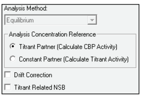
- Click the box to the left of “Drift Correction”.
- Analyze the data by pressing the “Analyze Data” icon.

Drift correction helps to decrease the percent error of the binding curve’s fit to the data points. Figure 1 shows a curve analyzed without drift correction (8.56% error) and Figure 2 shows the same curve with drift correction (1.76% error). Notice that the Kd and % Activity values changed only slightly due to the correction factor, but the bounds improved significantly. This is because when drifting data is analyzed using the standard model, the spread of the data is treated as random noise. The larger random noise gives a higher residual error which translates directly into greater uncertainty in the Kd or % Activity. Drift correction removes the systematic (i.e. not random) variation from the data resulting in a lower residual error and narrower confidence interval.

Figure 1. Example of a binding curve and error curve for an experiment measured without drift correction.

Figure 2. The binding curve and error curve for the experiment in Figure 1 measured with drift correction.
Frequently Asked Questions
Will drift correction correct for receptor instability?
No. An unstable receptor which is denaturing over time will exhibit a changing concentration and possibly a changing Kd as well. Neither of these effects is included in the drift correction.
Will drift correction correct the data for points measured before reaching equilibrium?
No. Non drifting samples measured before equilibrium may show pronounced drift-like changes in the middle of the curve but will not show similar systematic changes at the top and bottom of the curve. Figure 3 shows duplicate measurements of a system that is still proceeding towards equilibrium. Figure 4 shows duplicate measurements of a system that is at equilibrium but drifting. Drift correction directly affects the upper plateau of the curve (the Sig100 value) and the lower plateau of the curve (the NSB value) and should not be used when the changes in the data are only in the middle of the curve as in Figure 3.

Figure 3. An example of binding signals approaching equilibrium. Drift correction will not correctly model results from a system that is not at equilibrium.

Figure 4. Binding signals page showing systematic drift.
Details of Drift Calculations
Two drift terms are introduced to correct the data, “NSB drift” and “Signal drift”. The NSB drift is a linear drift and is given as millivolts (mV) per run. For example, if NSB is 0.100 V and NSB drift is -0.2 mV per run, the analysis theory would use 0.1 V for the first run, 0.0998 V for the second run, 0.0996 for the third run, and so on. See Table 1 for an example of NSB drift.
| Run # | NSB | NSB Drift per run |
|---|---|---|
| 1 | 0.1000 V | -0.0002 V |
| 2 | 0.0998 V | -0.0002 V |
| 3 | 0.0996 V | -0.0002 V |
| 4 | 0.0994 V | -0.0002 V |
Signal drift is exponential and is given as percent per run. To calculate the signal drift, the analysis examines the net signal instead of Sig100. Net signal is the difference between Sig100 and NSB. For example, if Sig100 is 1.0 V and NSB is 0.1 V, net signal is 1.0 V – 0.1 V or 0.9 V.
For an example of signal drift, assume the net signal is 0.9V and Signal drift is -1% per run. The second run would be 0.891 (0.9-0.009). The third run would be 0.88209 V (0.891-0.00891). See Table 2 for an example of how the software uses the drift correction on the signals.
| Run # | Net Signal | Signal Drift (based on -1% per run) |
|---|---|---|
| 1 | 0.9000 V | -(1% of 0.9000) = – 0.0090 V |
| 2 | 0.8910 V | -(1% of 0.8910) = – 0.0089 V |
| 3 | 0.8821 V | -(1% of 0.8821) = – 0.0088 V |
| 4 | 0.8733 V | -(1% of 0.8733)= – 0.0087 V |
Using the previous equation for net signal, the terms can be rearranged to obtain Sig100:
Since Sig100 includes both net signal and NSB, both drift terms affect the Sig100 value used. Table 3 shows the combined effect.
| Run # | NSB | Net Signal | Sig100 |
|---|---|---|---|
| 1 | 0.1000 V | 0.9000 V | 1.0000 V |
| 2 | 0.0998 V | 0.8910 V | 0.9908 V |
| 3 | 0.0996 V | 0.8821 V | 0.9817 V |
| 4 | 0.0994 V | 0.8733 V | 0.9727 V |