
Technology Note 213
Cooperativity
Cooperativity is a biomolecular interaction in which binding of a ligand to one site on a macromolecule influences binding at a second site. This Tech Note outlines the mathematics and implications of bivalent cooperativity using a bivalent IgG as an example. Cooperativity can either be positive, where the second binding event is tighter due to binding of the first ligand, or negative, where the second binding event is weaker.
Cooperative Equations
The diagram in Figure 1 shows a bivalent receptor (R) binding to a monovalent ligand (L). Referring to Figure 1, Kd1 and Kd2 can be mathematically expressed as Equations 1 and 2. Equations 3 and 4 simply state that the total receptor and total ligand are each equal to the sum of their bound and free components. With these equations the free fraction of receptor binding sites at equilibrium can be calculated.
Equation 1. Kd1 = [R][L] / [LR]
Equation 2. Kd2 = [LR][L] / [LRL]
Equation 3. RT = R + 2LR + LRL
Equation 4. LT = L + 2LR + 2LRL
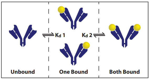
Figure 1. Diagram of cooperative binding.
Effect on Binding Curves
For a standard KinExA binding curve, one of the binding partners is kept constant (Constant Binding Partner or CBP) and the other binding partner is titrated (Titrant). Cooperativity may change the slope of the binding curve. The amount of change depends on the degree of cooperativity and the ratio ([CBP]/Kd) of the binding curve. A high ratio curve will be stoichiometric and therefore have little to no change. A low ratio curve will be influenced by cooperativity, with positive cooperativity making the curve steeper then it actually is and negative cooperativity making the curve more shallow.
When analyzing a single curve, cooperativity is very difficult to distinguish from a concentration error. For example, a binding curve with positive cooperativity is steeper than it is without cooperativity, but the noncooperative theory can still fit the data quite well by making the ratio higher than it actually is.
Figures 2A and 2B show cooperative data that is fit with the normal (noncooperative) binding theory. Both curves, when analyzed individually, fit the shape of the curve. Notice, however, that the calculated CBP activity in Figure 2A (187%) is much higher than 2B (78%). The CBP activity in Figure 2A is forced higher to increase the ratio thus increasing the slope of the binding curve. The higher curve (2B) is believable at 78% but the lower curve (2A) has a suspiciously high activity.
For a single curve, such as 2A, the high CBP activity could be due to a lower ligand activity than expected. With cooperativity though, the calculated activity of the CBP changes with the CBP concentration – higher ratios show lower activity, and lower ratio curves show higher activity.
Note: If the CBP is the reference concentration, the calculated Titrant activity changes in the other direction; higher ratios show higher ligand activity, and lower ratios show lower ligand activity.
The change in apparent activity with concentration provides a clue for identifying cooperativity. The same two curves from Figure 2 are analyzed as a noncooperative n-curve in Figure 3. Note the lower curve data (blue data points) has a steeper slope than the theory (blue solid line). This is because both curves are forced to the same activity of 75%. When this same data is analyzed using the cooperative theory (Figure 4) the fit is improved and the lower curve’s theory fits the slope of the data.
In Figure 4 the results are presented as an “Effective Kd” and “Hill Coefficient” rather than Kd1 and Kd2. The data is presented this way as an aid to intuitive understanding. Knowing that the Hill Coefficient is 1.76 and the effective Kd is 3.7 pM, we know the behavior of the system will be similar to a noncooperative system with a Kd of 3.7 pM, except low ratio curves will be steeper than expected. If, instead, the results are presented as Kd1 = 27 pM, and Kd2 = 500 fM it is difficult to construct an intuitive picture of the system’s behavior.

If you wish to find Kd1 and Kd2, they can be calculated from the Effective Kd (KdE) and Hill Coefficient using the following equations:
Equation 5.Kd1 = (KdE)(Hill) / (2 – Hill)
Equation 6.Kd2 = KdE(2 – Hill) / Hill
Confirmation of Cooperativity
Since cooperative binding causes a rather subtle deviation in the KinExA binding curves (seeFigure 3), it is prudent to confirm that this deviation from normal binding is caused by cooperativity rather than something else. Cooperativity can be confirmed by measuring the fill fraction (the fraction of antibodies with 0, 1, and 2 sites occupied) of equilibrated samples. This works because positive cooperativity suppresses the fraction of half filled antibodies compared to noncooperative binding.
Using Equations 1 through 4, the fractions of each species (one free, two free, or no free sites) can be calculated.Figure 5summarizes the binding distribution where the X axis is the Hill Coefficient and the Y axis is the fraction of total antibody, when the overall occupancy is 50%. As long as the total antibody sites are 50% occupied, the distribution at equilibrium changes with the degree of cooperativity, but not with the Kdor concentrations used to get the 50% occupancy.
InFigure 5notice that for a noncooperative antibody (Hill Coefficient of 1) half of the antibodies have one site occupied and a quarter of the antibodies have both sites bound. As positive cooperativity increases (Hill >1) the fraction of antibodies with one site occupied decreases finally reaching zero, for a Hill Coefficient of 2.
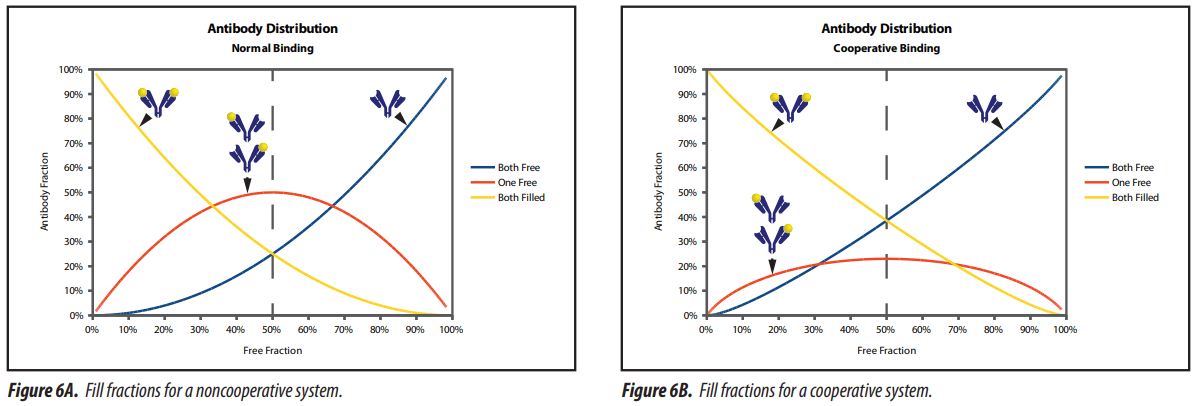
WhileFigure 5shows the fill fractions at 50% occupancy, as a function of the Hill Coefficient, it is also interesting to see the fill fractions as a function of occupancy.Figures 6A(noncooperative) and6B(cooperative) show the binding distribution as a function of the free fraction of total antibody binding sites. ComparingFigure 6Ato6Bshows that positive cooperativity suppresses the fraction of half filled antibodies at all occupancy levels.
Looking at the fill fractions in Figures 6A and 6B, the clearest difference between the cooperative and noncooperative system is at an occupancy of 50%, indicated by the dashed line. Knowing the fill fractions of an equilibrated sample makes it easy to tell if a system is truly cooperative when the occupancy is 50%.

Figure 5. Distribution of antibody filling as a function of Hill Coefficient when 50% of the available sites are filled.
The distribution can be inferred from the mass of the complexes formed in a mixture of bivalent antibody and its ligand. Mass spectrometry, using either MALDI or ESI, has sometimes been successfully applied to measure noncovalent complexes. Unfortunately the high charge ratios (often 30 or more for High Resolution MS) frequently cause the complexes to break apart. Ion-Mobility Spectrometry (IMS) uses a reduced charge electrospray ionization (charge ratio of 1) which results in a much easier analysis of noncovalent complexes. The resolution of the technique is poor compared to mass spectrometry and typically requires mass differences on the order of 10%. Therefore, when using this technique with an antibody, the ligand needs to have a molecular weight of about 15 kDa or more.
We identified a cooperative system with a ligand whose molecular weight is 28 kDa. We were also able to find a noncooperative antibody to the same ligand with a similar Kd. Samples were prepared at 50% occupancy and measured using the IMS instrument. Figure 7 shows the results of these measurements, in which suppression of the half filled antibodies is clear for the cooperative system.
The data in Figure 7B clearly shows there is cooperativity present. For this communication between the binding sites to take place, there must be a conformational change caused by binding of a ligand that is transmitted to the other binding site. For this to happen, the conformational change must extend at least to the hinge region, the closest common connection between the binding sites.

Figure 7. IMS measurement of both normal (noncooperative) and cooperative antibodies to the same ligand, when 50% of the binding sites are filled with ligand. Panel A is a noncooperative system, and panel B is a cooperative system.
There is some evidence of a conformational change extending well into the Fc region1. In the paper referenced, the binding change was caused by binding or modifying the Fc portion of the antibody. Since it is a common practice in Biacore measurements to capture the antibody on a chip using an anti-Fc capture antibody, it may be one of the reasons for the differences in Kd measurements between KinExA and Biacore.
Conclusion
Although cooperativity is not an uncommon occurrence, it is important to consider other reasons that may cause binding curves to exhibit cooperative traits. A concentration discrepancy between the curves in an n-curve analysis can appear as either positive or negative cooperativity. A mixture of clones in the CBP can appear as negative cooperativity. It is always a good idea to repeat the measurement if cooperativity is suspected.
If cooperativity is still suspected after ruling other causes out, independent confirmation can be attempted. However, independent confirmation uses much more material, is often difficult, and sometimes impossible. We are still working on better ways to diagnose and confirm cooperativity. Until there are other options available, the effective Kd measured is still the best way to understand the behavior of the system as a whole.
References
1. Blake II, R.C., et. al. 2005. Monoclonal antibodies that exhibit allosteric binding behavior. Trends in Monoclonal Antibody Research: Chapter I: 1-36