Newsletter #5

KinExA Analysis
When using KinExA Pro software to analyze data, only one binding partner’s concentration can be specified. The other concentration is calculated as part of the analysis and is reported as a percent activity. This is done to improve the accuracy of the reported Kd as described below.
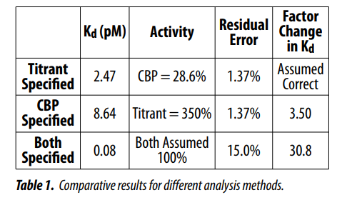
Although it is common to have the nominal concentration of both binding partners, the actual active concentration of the materials is often different than the nominal “known” concentration – sometimes substantially so. This is important because in KinExA analysis the accuracy of the Kd determination is proportional to the accuracy of the referenced binding partner concentration. This means a 30% error in the reference concentration will cause a 30% error in the Kd. However, it’s better than specifying both binding partner concentrations because in that case a 30% concentration error can lead to a much larger error in the Kd as shown in Table 1.
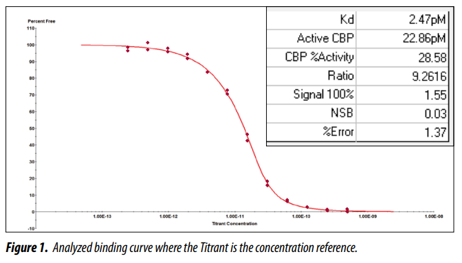
In Figure 1, the Titrant concentration is specified and the Constant Binding Partner (CBP) activity is calculated. The binding curve has a ratio ([CBP]/Kd) of 9 indicating sensitivity to both the CBP concentration and Kd. The theory fits the data well, resulting in a low residual error (1.37%). The measured activity for the CBP is calculated to be 28.6% which is a 3.5 fold decrease from the nominal “known” concentration supplied in the software. Plausible causes for a low activity include protein misfolding, insufficient purification, or a miscalculation in the nominal CBP concentration.
If we analyze the same data using the analysis method where the CBP is specified and the Titrant activity is measured the result is a change in Kd of 3.5 fold (Table 1). The change is directly proportional to the adjusted concentration of the CBP. The Titrant activity, at 350%, is also 3.5 fold higher than the previous analysis method. Unless there is a concentration error, it is uncommon for proteins to be over 100% active. In either case, the most the Kd will be affected is 3.5 fold.
If the same measured data is analyzed with both binding partners specified then the factor change in Kd is much larger (30.8 fold vs 3.5 fold, Table 1). The residual error is also greatly increased and there is no way to assess the activity of either binding partner since both are assumed to be 100%.
In the KinExA Analysis, the binding partner that is specified will depend on which one you trust more. If you are not sure, then look at the reported activity and decide if the result is reasonable. If the activity reflects over 100%, then specifying the other partner may be more appropriate.
Cooperativity
In our work with bivalent IgGs, we’ve found positive cooperativity to occur in about 5 to 10 percent of the antibodies we’ve studied. This fraction is in agreement with the published estimation by Dr. Blake (Blake II, R.C., et. al. 2005. Monoclonal antibodies that exhibit allosteric binding behavior. Trends in Monoclonal Antibody Research: Chapter 1: 1–36). We have yet to find a single confirmed case of negative cooperativity in antibodies.
If binding at the two sites is independent, binding at one site will not affect binding at the other site. With cooperative binding the first binding event (Kd1) will affect binding at the second site (Kd2). Cooperativity can either be positive, where the second binding event is tighter, or negative, where the second binding event is weaker.
For a standard KinExA binding curve, one of the binding partners is kept constant (Constant Binding Partner or CBP) and the other is titrated (Titrant). Cooperativity will show up as a change in the slope of the binding curve. The amount of change depends on the degree of cooperativity and the ratio ([CBP]/Kd) of the binding curve. A high ratio curve will be stoichiometric and therefore have little to no change. A lower ratio curve will be influenced with positive cooperativity making the curve steeper than it actually is and negative cooperativity making the curve more shallow.
Figures 2A and 2B show cooperative data that is fit with the normal (noncooperative) binding theory. Both data sets, when analyzed individually, fit the shape of the curve. Notice, however, that the calculated CBP activity in Figure 2A (187%) is much higher than 2B (78%). The CBP activity in Figure 2A is forced higher in the analysis to increase the ratio thus increasing the slope of the binding curve. The higher curve (2B) is believable at 78% but the lower curve (2A) has a suspiciously high activity.
For a single curve, such as 2A, the high CBP activity could be due to a lower Titrant activity than expected. With cooperativity though, the calculated activity of the CBP changes with the CBP concentration – higher ratios show lower activity, and lower ratios show higher activity.
Note: If the CBP is the reference concentration, the calculated Titrant activity changes in the other direction; higher ratios show higher Titrant activity, and lower ratios show lower Titrant activity.
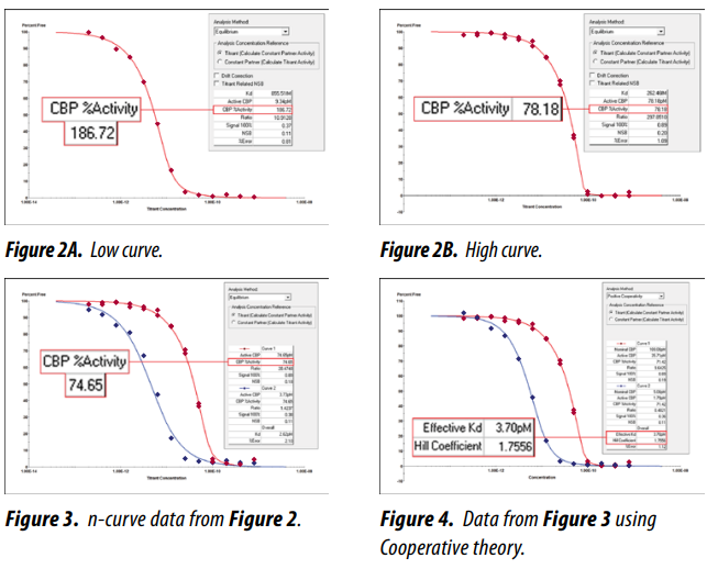
The change in apparent activity with concentration provides a clue to identifying cooperativity. The same two curves from Figures 2A and 2B are analyzed as an n-curve in Figure 3. Note the lower curve data (blue data points) has a steeper slope than the theory (blue solid line). This is because both curves are forced to the same activity of 75%. When this data is analyzed using the cooperative theory (Figure 4) the fit of the theory to the lower curve data is improved.
In Figure 4 the results are presented as an “Effective Kd” and “Hill Coefficient” rather than Kd1 and Kd2. The data is presented this way as an aid to intuitive understanding. In Figure 4, knowing the Hill Coefficient is 1.76 and the effective Kd is 3.7 pM, we know the behavior of the system will be similar to a noncooperative system with a Kd of 3.7 pM, but the lower curve will be a bit steeper. If, instead, the results are presented as Kd1 = 27 pM, and Kd2 = 505 fM it is difficult to construct an intuitive picture of the system’s behavior.
Kd1 and Kd2 can be calculated from the Effective Kd (KdEff) and Hill Coefficient (Hill) using the following equations:

For more information refer to Tech Note 213 Cooperativity (TN213).
Spotlight: EZ Align Tool
We are pleased to introduce the EZ Align lamp alignment tool (Part #: 800510). This new device has a fluorescent target that snaps in place of the flow cell enabling simple lamp alignment. Optimal lamp alignment equals maximum signal output.
Features
- Integrated software provides a real time voltage graph that guides lamp alignment towards peak performance.
- Small, lightweight, and durable
- 10 year warranty
- Compatible with software versions 4.2.4 and newer
We encourage you to order the EZ Align tool for a simple and intuitive way to achieve optimum lamp alignment. Please visit www.sapidyne.com for more details.
Ask the Inventor
Question
How can I confirm my antibody is really cooperative?
Answer
What a good question! The inventor shares and encourages the skepticism that underlies it.
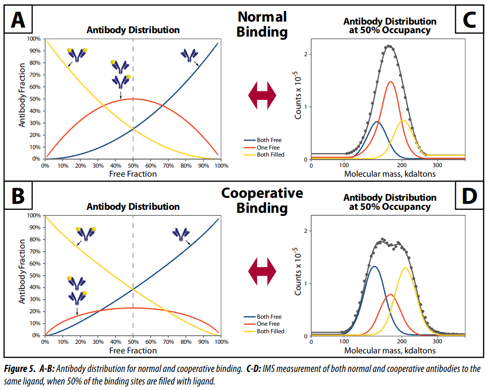
As is often the case, we look for an orthogonal measurement that also shows cooperativity for the same antibody. The measurement we’ve identified is the mass distribution of the antibody-ligand complexes. This works because cooperative binding causes a change in the relative abundance of doubly bound, singly bound, and unbound antibody.
Consider first a noncooperative bivalent antibody binding to a monovalent ligand in solution. Imagine we have selected antibody and ligand concentrations such that, at equilibrium, half of the antibody binding sites are occupied by ligand. This means the probability that any given antibody binding site is occupied is 0.5. For a noncooperative system with a 50% antibody occupancy the fraction of the antibody that is doubly bound is 25%, singly bound is 50%, and unbound is 25%. This distribution is shown graphically along the dashed line in Figure 5A.
Next consider an antibody that is positively cooperative, meaning when the first site binds the second site becomes more likely to bind. This cooperativity shifts the distribution of the bound sites. At the same 50% bound condition there will be more than 25% of the antibodies with both sites bound and less than 50% of the antibodies will have one site bound, see the distribution along the dashed line in Figure 5B. Comparing Figure 5A to 5B shows that positive cooperativity suppresses the fraction of half filled antibodies at all occupancy levels.
The distribution can be estimated from measurements of the mass of the complexes formed in a mixture of bivalent antibody and its ligand. Mass Spectrometry (MS), using either Matrix-Assisted Laser Desorption/Ionization (MALDI) or Electrospray Ionization (ESI), has sometimes been successfully applied to measure noncovalent complexes. A downfall of those techniques is that the high charge ratios (30 or more for High Resolution MS) often cause the complexes to break apart. Ion Mobility Spectrometry (IMS) uses a reduced charge electrospray ionization (charge ratio of 1) resulting in a much easier analysis of noncovalent complexes. The resolution of this technique is poor compared to MS and typically requires mass differences on the order of 10%. Therefore, when using this technique with an antibody, the ligand needs to have a molecular weight of about 15 kDa or more.
We identified a cooperative system with a ligand whose molecular weight is 28 kDa. We were also able to find a noncooperative antibody to the same ligand with a similar Kd. Samples were prepared at 50% occupancy and measured using the IMS instrument. Figures 5C and 5D show the results of these measurements, in which the suppression of the half filled antibodies is clear for the cooperative system.
The data in Figure 5D clearly shows a binding distribution consistent with cooperativity. Additional information and literature references can be found in Tech Note 213 Cooperativity (TN213).
Tips & Tricks
Reusing Beads
To define a system’s Kd, kinetics, and active binding site concentration three vials of PMMA beads (Part #: 440176) or one and a half vials of Azlactone beads (Part #: 444110) are typically needed. Each vial requires between 10 to 30 μg of material to adequately coat the surface of the beads. To help save time and coating material Sapidyne has developed bead retrievers for both the KinExA instrument and Autosampler.
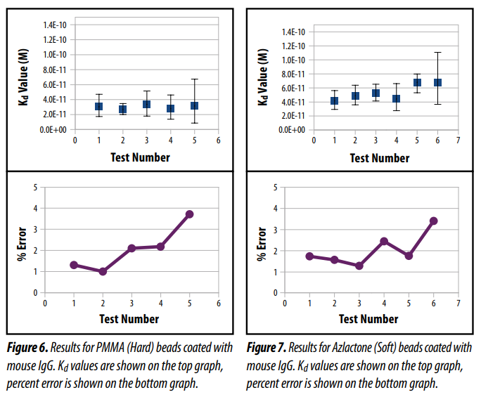
Typically only a small percentage of binding sites on the beads are bound in one experiment. This means there are still binding sites available on the beads for future experiments. In testing both hard and soft beads we found that we could capture and reuse the beads several times before seeing any significant changes to the data. The number of times the beads can be reused varies depending on the system. When recycling beads, be mindful of any changes to the data such as system noise, percent error, signal level, and non specific binding (NSB). With reuse, signal level tends to decrease while noise, error, and NSB increase.
To demonstrate, mouse IgG was used to coat both PMMA and Azlactone beads. Each bead type was reused four times before the residual error exceeded 3% (See Figures 6 and 7). Even with increased error, all curves maintained overlapping 95% confidence intervals for the measured Kd.
The KinExA Bead Retriever (Part #: 393100) is compatible with any version of the software, while the Autosampler Bead Retriever (Part #: 393120) is compatible with versions 3.3.0 and newer. For more information see Tech Note 226 Reusing Beads (TN226). Please refer to our website under Parts & Consumables > Accessories for pricing on the retrievers.