Newsletter #4

KinExA Mode
In KinExA® experiments, samples containing a mixture of two binding partners (along with their complex) are briefly exposed to a solid phase coated with one of the binding partners.
Kinetic Exclusion Assay refers to the underlying principle that contact time between any portion of the sample to the solid phase is short enough that dissociation of the sample’s molecular complex is insignificant. Experiments run under these conditions are said to be in “KinExA Mode.” This article will briefly outline how to determine if your experiments are in KinExA Mode.
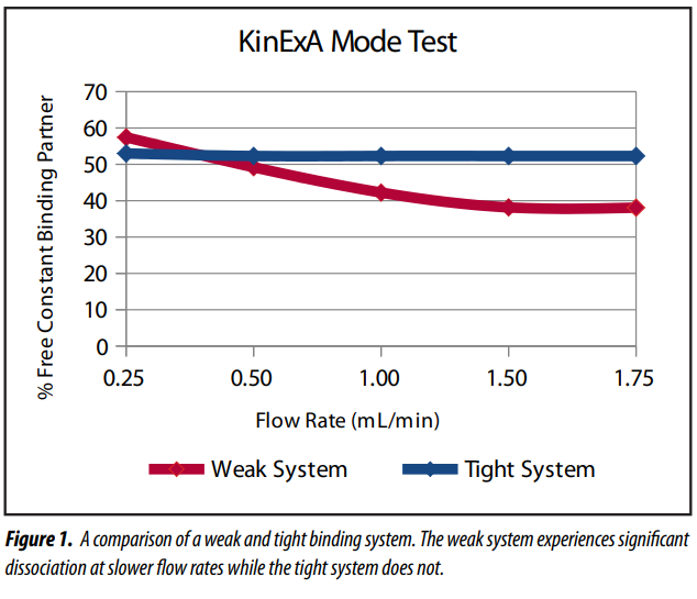
When a system is out of KinExA Mode there is significant dissociation of the sample complex and the solid phase captures not only free constant binding partner (CBP) but CBP that has dissociated from the titrant. This results in an elevated signal and a falsely high estimate of the percent free CBP. An easy test can be conducted to determine if a system is in KinExA Mode. The test compares a single point of inhibition (ideally ~50% free CBP) to determine if the percent free CBP decreases as flow rate increases. Because signals vary with flow rate, an uninhibited point (Sig 100%) and a point near full inhibition (NSB) is needed to calculate the percent free CBP.
Figure 1 displays a comparison between a weak system that was not in KinExA Mode and a tight system that was in KinExA Mode. For the weak system the percent free CBP drops from ~58% free at 0.25 mL/min to ~39% free at 1.5 mL/min (the flow rate at which the weak system has finally entered KinExA Mode). The tight system shows multiple flow rates in KinExA Mode for illustrative purposes only. If a significant change in percent free CBP is not observed as the flow rate is increased, further testing is not necessary.
KinExA Mode tests can be performed prior to running equilibrium experiments if preliminary range find results indicate a Kd weaker than single digit nanomolar. When running Kinetic Exclusion Assays at the default 0.25 mL/min flow rate the contact time of the sample to the solid phase is ~0.5 seconds. Most systems with a single digit nM Kd or tighter will be in KinExA Mode at the default flow rate. Weak systems can be brought back into KinExA Mode by increasing the flow rate, which shortens the contact time. See Tech Note 221 KinExA Mode (TN221) for more information.
Hints & Tricks
Reducing NSB
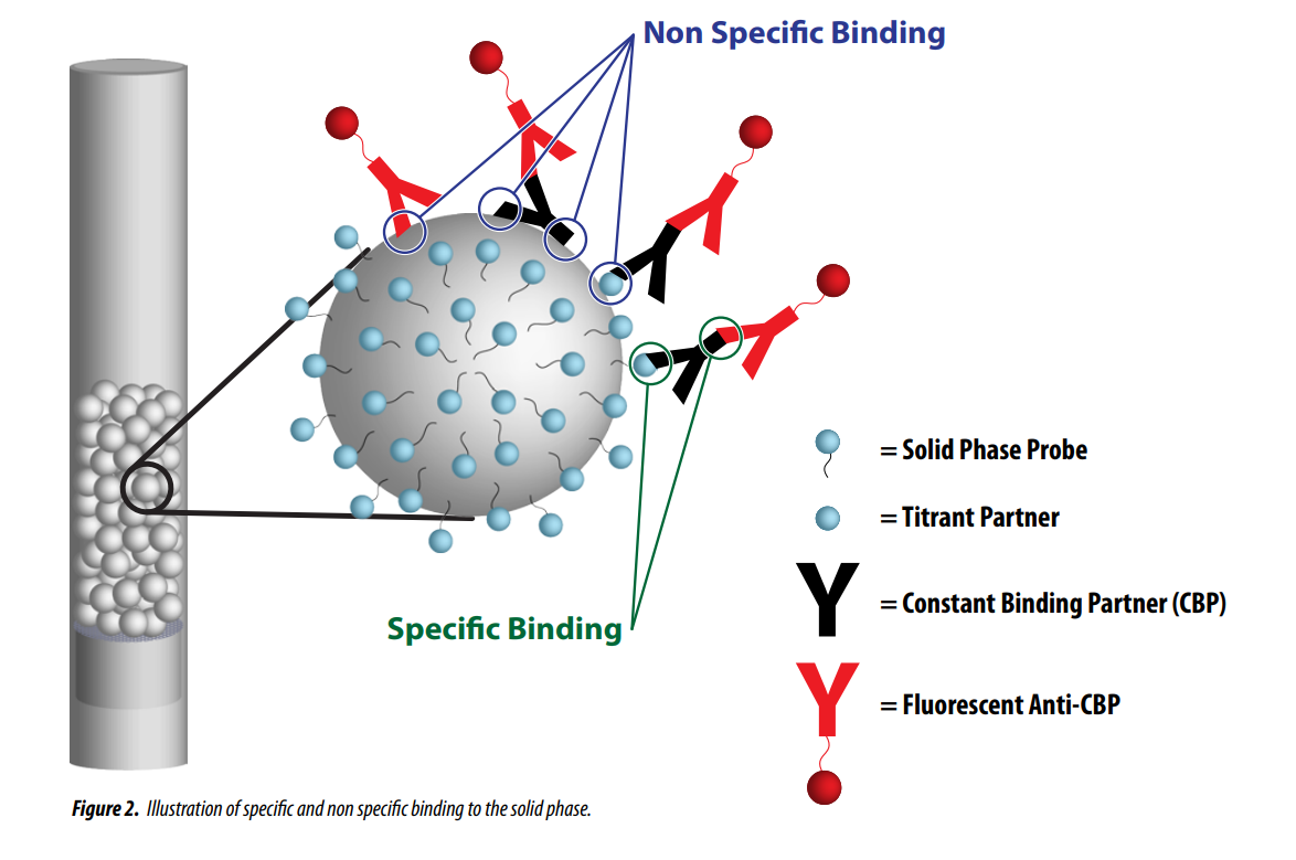
Specific binding is the binding of a constant binding partner’s (CBP) active site to its target on the titrated binding partner. Non specific binding (NSB) is any other binding that occurs in the system that interferes or adds to the specific binding and complicates the measurement.
Although NSB is accounted for in the analysis and subtracted from the signals, noise still contributes to greater uncertainty in the measurements. If NSB is a significant percent of the total signal, it is worth the effort to reduce it before continuing.
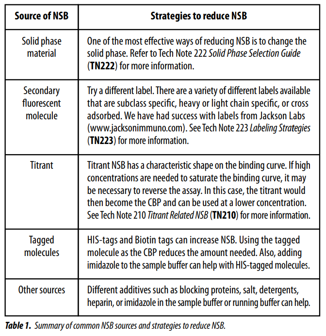
The first step in reducing NSB is to identify and understand the source of NSB. Table 1 summarizes common sources and strategies to reduce NSB. For more information, refer to Tech Note 219 Reducing Non Specific Binding (TN219).
Note: Some NSB strategies may interfere with one another so it is best to try them individually.
Ask the Inventor
Question
The only way I can increase my signal is to run very high volumes. The large samples make painfully long experiment run times. Is there anything else I can do to optimize my signal?
Answer
Increase your signal to what? Everyone, including me, likes big signals but what actually impacts data quality is not the signal level but the signal to noise ratio. My suggestion is don’t increase your signal. You may significantly increase material needed and run time without any gain.
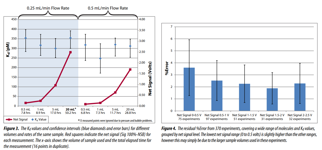
To demonstrate the practicality of this approach, I ran a series of experiments in which I prepared very large volumes of titrated ligand-antibody mixtures. I split each of the 16 titrations into eight separate sets of tubes and then ran duplicate volumes of 20 mL, 5 mL, 1 mL, and 0.5 mL at 0.5 mL/min and 0.25 mL/min. The antibody I used was a commercially available mouse anti-insulin and the solid phase was azlactone coated with insulin. The results are summarized in Figure 3.
As you can see, the confidence intervals for the Kd values all show substantial overlap even though net signals vary from 0.09 to 2.8 volts, run times range from 6.8 to 50.2 hours, and sample material usage varies 40 fold.
A further investigation of 370 experiments found that over half (52%) had a net signal of less than 1 volt and 24% had a net signal of less than 0.5 volts. The %Error had more variability at the smallest signal levels, but many had a low %Error (2% or less). In Figure 4 I’ve grouped the signals into ranges and show the average %Error and the standard deviation in the %Error for each group.
The average %Error for the lowest signal range is significantly higher, statistically, than the other signal ranges. Differences between the other ranges are marginal or insignificant. Sample volume information was not available in this data extraction but it is likely that many of the small signal experiments also included large volumes which may have contributed to the higher %Error values.
My suggestion is that if your signal is less than 0.5 volts and your sample volume is less than 5 mL, go ahead and increase your volume up to 5 mL or until your signal is over 0.5 volts. As a rule, don’t go over 5 mL sample volumes. Larger volumes frequently lead to clogging related pressure problems (I had to ignore 13 points in one of my 20 mL experiments and I changed the flow cell after both 20 mL experiments due to pressure increases). Overall, I believe your chance of success is higher with a smaller signal than with 10 or 20 mL sample volumes.
Note: If you are interested in seeing the experiment files behind Figure 3 you can download them from www.sapidyne.com under the Downloads section.