Introduction to Reversible Binding
“The first step in essentially all biological activities is a union between separate constituents into a merged entity.” In the context of biochemistry, binding is the joining of two entities (molecules) that have some affinity for each other. This binding is almost always reversible, meaning the two molecules (generically known as ligand and receptor) will join together and come apart over and over again.
Binding Constants
Equilibrium
Receptor and ligand associate (bind), remain linked together for a while, and then dissociate (come apart). Eventually, an equilibrium state is reached such that the concentration of bound partners is no longer changing. Association and dissociation continue, but since the concentrations are no longer changing, the number of association events per second must equal the number of dissociation events per second.
Kinetics and Affinity
The rate at which the molecules associate is proportional to the concentrations of the molecules. If the concentration of either the ligand or the receptor is doubled, the rate of association is also doubled. Mathematically we write this as:
The term “kon” is a constant of proportionality and is known as the “on rate” for the particular receptor and ligand under study. Likewise, the rate of dissociation is proportional to the concentration of the receptor ligand complex. The constant of proportionality "koff" is known as the “off rate”:
This ratio is called the equilibrium dissociation constant and is represented by the term Kd. It is closely related to the equilibrium association constant, which is represented by the term K, or sometimes Ka. Kd and K are the inverse of each other:
Historically, the term “affinity” referred strictly to the equilibrium association constant (K). Currently, binding constants are often given in terms of Kd rather than K. This is because the units of Kd are concentration (M) and therefore much more intuitive than inverse concentration (M-1), the units of K. Now the term “affinity” often refers to Kd instead of K. A colleague may say, “The affinity of this antibody is low nanomolar.” Obviously, the speaker is actually referring to the Kd rather than the K because the units are in terms of concentration. This distinction is being highlighted because of the ambiguity created when using the relative terms “high” and “low” associated with the term affinity. Ambiguity can be eliminated by using the relative terms “tight” and “weak” rather than “high” and “low” when speaking about affinity.
|
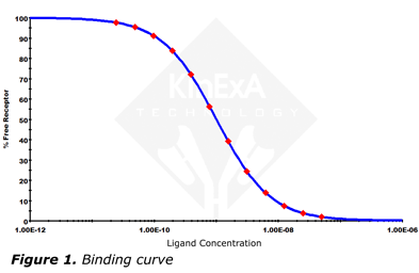
A useful way to illustrate binding is to look at binding curves. Usually they are plots of either the free or bound fraction of one component, versus the concentration of the other component. The most useful type of plot is semilogarithmic (Figure 1).
The equation to generate this plot only needs Kd and the total receptor concentration, [RT]. Depending on the values of Kd and [RT], the curve shape and location on the [LT] axis can change. By using the ligand concentration at 50% free receptor, [L50], as the location indicator, it can be described by the simple equation: 
|
|
|
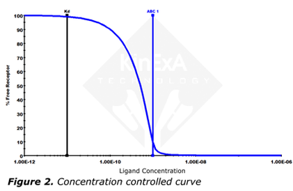
The shape of the curve is completely defined by the ratio [RT]/Kd. A high ratio curve (above about 10) is called a concentration controlled curve, is steeper, and has a relatively sharp lower knee (Figure 2). A concentration controlled curve is mostly dependent on the concentration of receptor ([RT]) and has little dependence on Kd |
|
|
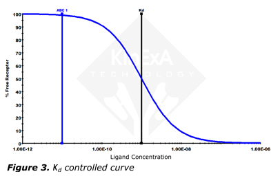
A low ratio curve (near or below 1) is called a Kd controlled curve, is less steep, and has a more gentle lower knee (Figure 3). A Kd controlled curve is mostly dependent on Kd and has little dependence on receptor concentration.
|
|
At equilibrium the total association events equal the total dissociation events, so the equation may be written:
Where:
kon= association rate constant
[R] = free receptor site concentration
[L] = free ligand site concentration
koff = dissociation rate constant
[RL] = concentration of complex
Since Kd is koff/kon, equation (1) may be rewritten:


Both sides are multiplied by a common factor (1/[RT]) to get the equation in terms of free fraction or [R]/[RT] (11):

Klotz I.M. 1997. Ligand-receptor energetics: a guide for the perplexed. New York: John Wiley & Sons, Inc. https://books.google.com/Ligand-receptor energetics...
Ohmura N., Lackie S., Saiki H. 2001. An immunoassay for small analytes with theoretical detection limits. Anal Chem 73: 3392-3399. http://www.ncbi.nlm.nih.gov/pubmed/11476240